This is the multi-page printable view of this section. Click here to print.
Articles
Color mapping for data visualization
Jupyter notebook:
A Jupyter notebook with the code in this article is available in Google Colab. Check it out!Introduction
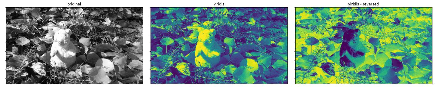
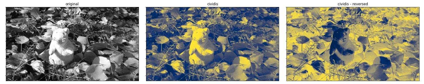
Data visualization is an important tool for presenting the results of new algorithms. For 2D data in particular, it is possible to visualize the data as colored images so that our brains can interpret the data in a visual way. This article presents new color mapping nodes available in Lluvia to transform 2D data into color images. These nodes use several color maps available in the Matplotlib project to accelerate data to color conversion using the GPU.
Color mapping
Let $F : \mathbb{Z}^{2}_{\ge 0} \rightarrow \mathbb{R}$ be a scalar field defined for $(x, y)$ in the set of integer numbers greater or equal zero (standard image coordinates). The value $F(x, y)$ on each point is an element of the real numbers $\mathbb{R}$.
Next, let $c(z) : \mathbb{R} \rightarrow \text{RGB}$ be a color mapping function converting from a real value $z$ to RGB color space. In practice, the color output of $c(z)$ must be in a closed range that enables visualization in a computer screen. Constraining each color component to lie in the range $[0, 255]$ is common. This can be achieved by limiting the range of the input $z$ to values in the interval $[0, 1]$, that is:
$$ \bar{z} = \frac{z}{z_\text{max} - z_\text{min}} $$
where $z_\text{min}$ and $z_\text{max}$ are known values.
The color field $C : \mathbb{Z}^{2}_{\ge 0} \rightarrow \text{RGB}$ is the result of applying the color mapping function of all values of field $F$ as:
$$ C(x, y) := c\left( \frac{F(x, y)}{z_\text{max} - z_\text{min}} \right) $$
Gray color mapping
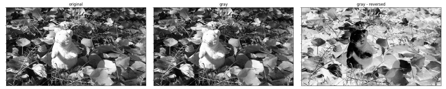
A simple color mapping function is the one mapping to gray scale values. $c_\text{gray}(z)$ is defined as:
$$ c_\text{gray}(\bar{z}) = 255 (\bar{z}, \bar{z}, \bar{z}) $$
That is, creating a 3-vector of the normalized input value repeated in each color component and multiplying it by 255 to obtain an RGB color.
Complex color mappings
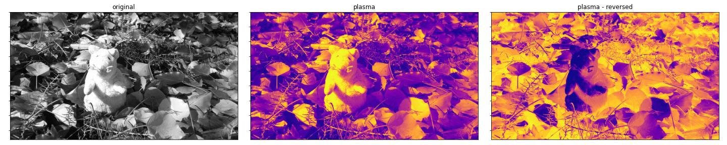
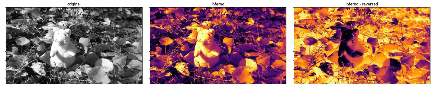
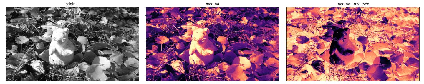
More complex color maps have a whole set of research on color theory, human color perception and physics. Designing new color maps exclusive for Lluvia is out of scope for the project and serves little purpose as there are great color maps readily available from the open source community. In particular, since I work with Python a lot, and use Matplotlib heavily, I decided to export several of the color maps available there into Lluvia. The reader is highly encouraged to watch the presentation below from Stéfan van der Walt (@stefanv) and Nathaniel Smith (@njsmith) on a default perceptually uniform colormap for Matplotlib.
The following color maps are extracted from Matplotlib using code similar to that presented in the Appendix section:
- Perceptually uniform maps:
- viridis.
- plasma.
- inferno.
- magma.
- cividis.
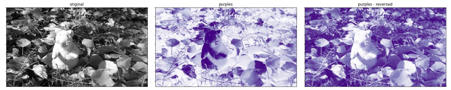
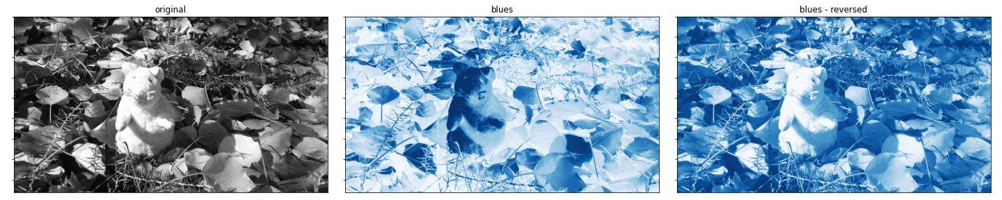
- Sequential maps:
- gray.
- purples.
- blues.
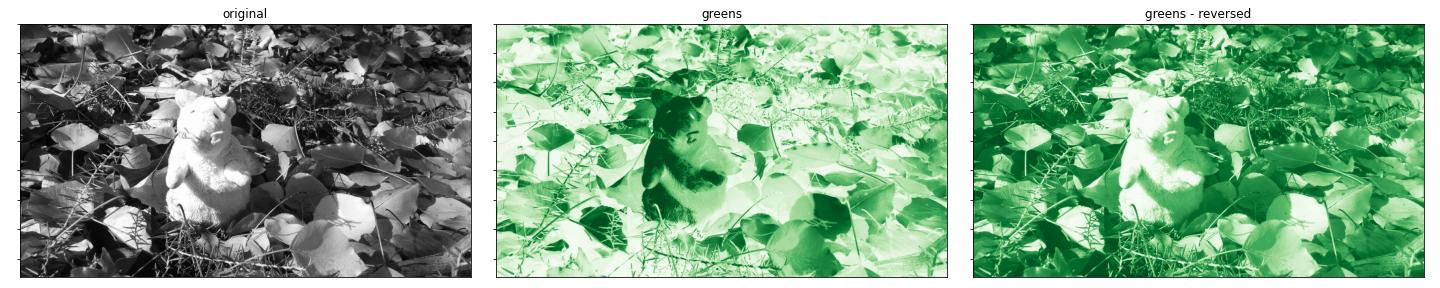
- greens.
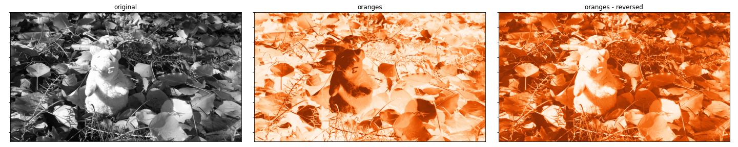
- oranges.
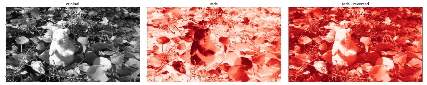
- reds.
- Diverging maps:
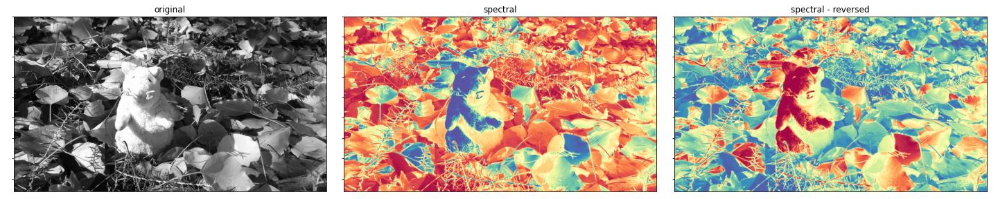
- spectral.
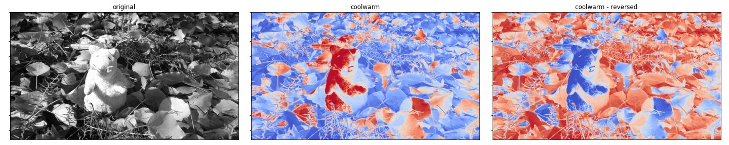
- coolwarm.
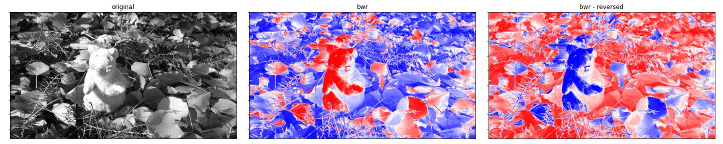
- bwr.
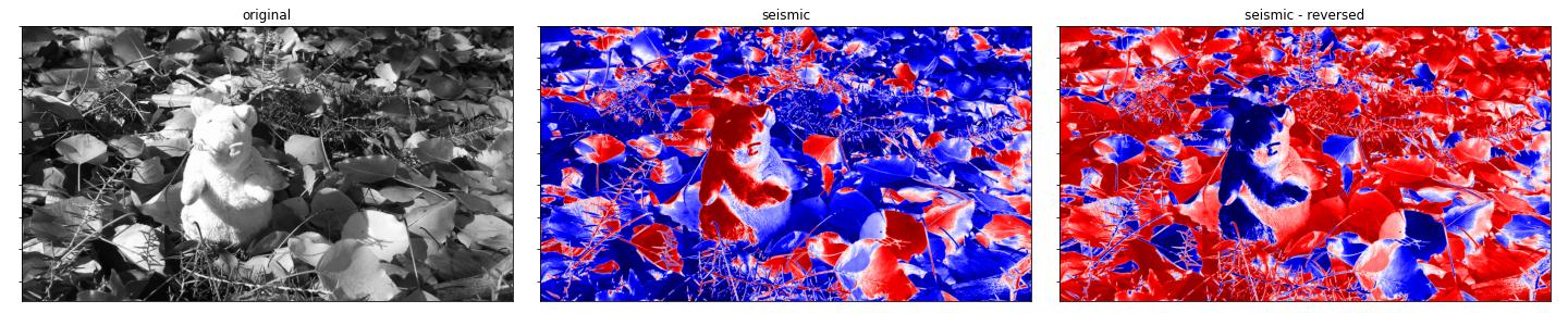
- seismic.
- Cyclic maps:
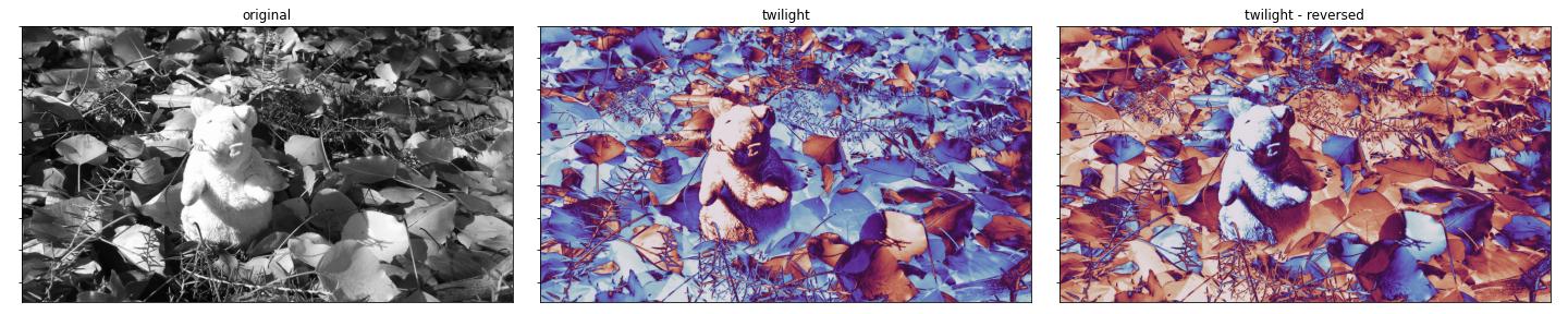
- twilight.
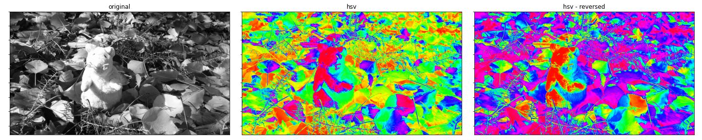
- hsv.
Colormap nodes in Lluvia
There are four new nodes available in Lluvia for color mapping:
lluvia/viz/colormap/ColorMap             : Container : Maps a scalar field to a color field using a color map.
lluvia/viz/colormap/ColorMap_float       : Compute   : Maps a floating point scalar field to a color field using a color map.
lluvia/viz/colormap/ColorMap_int         : Compute   : Maps an integer scalar field to a color field using a color map.
lluvia/viz/colormap/ColorMap_uint        : Compute   : Maps an unsigned integer scalar field to a color field using a color map.
ColorMap_float, ColorMap_int, and ColorMap_uint process input fields of float, int, and uint types respectively. They are aggregated by the ColorMap container node (no suffix), which instantiates one of the others according to the input image type.
The interface of ColorMap is:
- Parameters:
color_map: string. Defaults to “viridis”.min_value: float. Defaults to 0.0. Minimum input value.max_value: float. Defaults to 1.0. Maximum input value.alpha: float. Defaults to 0.0. The alpha value of the output image in range [0, 1].reverse: float. Defaults to 0.0. If 1.0, the color map is reversed.
- Inputs:
in_image: ImageView. {r8ui, r16ui, r32ui, r8i, r16i, r32i r16f, r32f} image. Input image.
- Outputs:
out_image: ImageView. rgba8ui image. The encoded color of the optical flow field.
The code bellow shows how to instantiate, configure, and run the ColorMap node:
| |
Perceptually uniform maps
viridis
plasma
inferno
magma
cividis
Sequential maps
gray
purples
blues
greens
oranges
reds
Diverging maps
spectral
coolwarm
bwr
seismic
Cyclic maps
twilight
hsv
Appendix
Color map extraction from matplotlib
| |
which produces an output similar to
builder.colorMaps['viridis']  = 'RQJVAEUDVgBFBFgARgZZAEYHWwBGCVwARwpdAEcMXwBHDWAARw9iAEgQYwBI...'
builder.colorMaps['plasma']   = 'DQiHABEIiAAUB4oAFgeLABkHjAAcB40AHgeOACAGjwAiBpAAJAaRACYGkgAo...'
builder.colorMaps['inferno']  = 'AQEEAAEBBQABAQcAAgEIAAICCgACAgwAAwIPAAMDEQAEAxMABQQVAAUEFwAG...'
builder.colorMaps['magma']    = 'AQEEAAEBBQABAQcAAgEIAAICCgACAgwAAwMOAAMDEAAEBBIABQQUAAUFFgAG...'
builder.colorMaps['cividis']  = 'ACNOAAAkUAAAJFEAACVTAAAmVQAAJ1YAACdYAAAoWgAAKVwAACldAAAqXwAA...'
builder.colorMaps['gray']     = 'AAAAAAEBAQACAgIAAwMDAAQEBAAFBQUABgYGAAcHBwAICAgACQkJAAoKCgAL...'
builder.colorMaps['purples']  = '/Pv9APz7/QD8+/0A+/r9APv6/AD6+fwA+vn8APr4/AD5+PsA+fj7APj3+wD4...'
builder.colorMaps['blues']    = '9/v/APf7/wD2+v8A9fr/APT5/gD0+f4A8/j+APL4/gDx9/0A8Pf9APD2/QDv...'
builder.colorMaps['greens']   = '9/z1APf89QD2/PQA9vz0APX88wD1+/IA9PvyAPT78QDz+/AA8vvwAPL67wDx...'
builder.colorMaps['oranges']  = '//XrAP/16wD/9eoA//TpAP/06AD/8+cA//PmAP/y5QD/8uQA//HjAP/x4gD/...'
builder.colorMaps['reds']     = '//XwAP/18AD/9O8A//TuAP/z7QD/8uwA//LrAP/x6gD/8OkA//DoAP/v5wD/...'
builder.colorMaps['spectral'] = 'ngFCAKEEQwCjBkQApQlEAKcLRQCpDUUAqxBGAK4SRgCwFUcAshdHALQZSAC2...'
builder.colorMaps['coolwarm'] = 'O03BADxOwgA9UMQAP1LFAEBUxwBBVcgAQlfKAENZywBEW80ARlzOAEde0ABI...'
builder.colorMaps['bwr']      = 'AAD/AAIC/wAEBP8ABgb/AAgI/wAKCv8ADAz/AA4O/wAQEP8AEhL/ABQU/wAW...'
builder.colorMaps['seismic']  = 'AABNAAAAUAAAAFMAAABVAAAAWAAAAFsAAABeAAAAYQAAAGMAAABmAAAAaQAA...'
builder.colorMaps['twilight'] = '4tnjAOHa4wDg2uIA39rhAN7a4QDc2eAA2tnfANnY3gDX190A1dfcANPW2wDQ...'
builder.colorMaps['hsv']      = '/wAAAP8GAAD/DAAA/xIAAP8YAAD/HgAA/yQAAP8qAAD/MAAA/zYAAP88AAD/...'
Raspberry Pi 4 build
Introduction
The Raspberry Pi 4 project announced back in November 2020 that the Vulkan 1.0 conformance tests successfully passed for its GPU driver. More recently in August 2022, Vulkan 1.2 conformance testing has been completed.
The conformance tests are a large set of tests run against a driver implementation to see if it conforms with the Vulkan specification. This is essential to maintain the Vulkan API portable across platforms and GPU vendors.
In addition, LunarG announced support of the Vulkan SDK on the Raspberry Pi 4. With this, the two most important requirements to build Lluvia on the RPi4 became available.
Build instructions
The build instructions are available in the Getting started page. They can be summarized as:
- Prepare the operating system.
- Build the Vulkan SDK following the official documentation.
- Build and install OpenCV (for running demos).
- Install Bazel.
- Build and install Lluvia.
Optical flow demo
There is a new demo shipped with the Lluvia source code to run pipelines with images captured from a camera. Currently, the demo uses OpenCV VideoCapture class to capture images from the Raspberry camera module.
The demo app, which can be run from the repository root folder as
| |
configures the camera to capture images at 320x240 resolution and runs the webcam/HornSchunck container node defined in the horn_schunck.lua script. The container node creates the pipeline illustrated below:
@startuml
skinparam linetype ortho

state BRGA2Gray
state HS as "HornSchunck"
state Flow2RGBA
state RGBA2BGRA

BRGA2Gray -down-> HS: in_gray
HS -down-> Flow2RGBA: in_flow
Flow2RGBA -down-> RGBA2BGRA: out_rgba
@enduml
with the HornSchunck node containing the algorithm implementation as discussed in a previous article.
OpenCV BGR color ordering
By default, OpenCV used BGRA channel ordering for color images. On the other hand, Lluvia uses RGBA ordering to store color images. The last node in the demo pipeline converts to the color order OpenCV expects to render into the screen.Discussion
This post introduced the instructions for building Lluvia on the Raspberry Pi 4. A new demo application for running pipelines with images captured from the Pi’s camera module is also presented.
As of now, Lluvia is supported in four platforms:
- Linux x86_64.
- Windows.
- Android through the mediapipe integration.
- Raspberry Pi 4.
Future work can include support for other platforms such as:
- Nvidia Jetson hardware.
- MacOS and iOS.
With these many platforms, an interesting topic for future work is running benchmarks across all of them for assessing the runtime performance of different computer vision algorithms.
Android integration using mediapipe
Introduction
The previous post on mediapipe integration explored how to integrate Lluvia with Mediapipe to create complex Computer Vision pipelines leveraging mediapipe’s integration with other frameworks such as OpenCV and Tensorflow. This post expands this integration to run Lluvia on Android systems.
The video below shows the Optical Flow Filter algorithm running on a Samsung Galaxy S22+ phone.
Graph for mobile applications
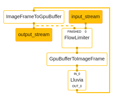
The figure below illustrates the pipeline used on Android for running the LluviaCalculator. First, a FlowLimiter calculator receives the images from the input_stream. This calculator controls the rate at which packets are sent downstream; it receives an additional input from the last calculator, ImageFrameToGpuBuffer, that indicates processing has been completed and that a new packet can be received.
The GpuBufferToImageFrame and ImageFrameToGpuBuffer calculators convert packets from GpuBuffer to ImageFrame and vice-versa. They are needed for two reasons:
- On Android, the
input_streamandoutput_streamports of the pipeline expectGpuBuffertypes. - Currently, the
Lluviacalculator cannot handleGpuBufferpackets.
Finally, the Lluvia calculator runs the configured GPU pipeline.
GpuBuffer support
Support for transferring data to and fromGpuBuffer packets in the LluviaCalculator is planned. This will avoid the use of GpuBufferToImageFrame and ImageFrameToGpuBuffer calculators, thus reducing the memory copy overhead.Android application
The mediapipe repository provides examples on how to build Android applications that run the framework. The dataflow is as follows:
- In Java/Kotlin, configure the app to open the camera. Camera2 or CameraX APIs can be used.
- Camera frames are received on Surface objects, opaque objects that hold reference to the image pixel data.
- The surface objects are transferred to the mediapipe graph, entering through the
input_stream. In there, the packets are sent asGpuBufferto be consumed by the calculators. - The graph execution takes place, and the output packets are received by the application through the
output_stream. TheGpuBufferpackets are transformed to Android surface objects. - The surface objects are rendered in the screen.
Mediapipe Android archive
Build instructions
The mediapipe integration guide includes new instructions on how to configure the project to support Android builds.Apps can consume medipipe libraries through Android Archive files (AAR). Archives are a special type of library containing JVM classes, assets, and native libraries (compiled for x86, arm64, or other architectures). Archives can be imported to the app either by placing them within the app source tree, or by declaring a dependency to a remote repository (e.g. Maven).
Mediapipe bazel rules include targets to build AAR files than be used on Android. The lluvia-mediapipe repo uses these rules to compile an archive that compiles lluvia along with mediapipe, and export all the required assets (node library, scripts and graphs). The AAR is created by running:
| |
where --fat_apk_cpu=arm64-v8a defines the CPU architectures that the native code will be compiled to. The archive is available at:
bazel-bin/mediapipe/lluvia-mediapipe/java/ai/lluvia/lluvia_aar.aar
which can directly be copied to the App’s libraries, or exported to a remote repository.
Discussion
This post explained how to use Mediapipe to run Lluvia compute pipelines on Android systems. The mobile graph uses the FlowLimiter calculator to control the rate at which image packets are consumed by the pipeline. Future work includes:
- Support
GpuBufferinput and output packets in theLluviacalculator. - Fully working Android code example.
- Use the Android GPU Inspector to profile the performance of the app.
Mediapipe integration
Introduction
Mediapipe is a cross-platform framework to create complex Computer Vision pipelines both for offline and real-time applications. It leverages popular frameworks such as OpenCV and Tensorflow to process audio, video, and run deep learning models. By integrating Lluvia into mediapipe, it is possible to speed up some of those computations by creating a GPU compute pipeline.
Difference 1: project scope
Mediapipe is a more general framework than Lluvia. Mediapipe, at its core, is a compute graph scheduler, where each node can contain any arbitrary processing logic. The integration of third-party frameworks (e.g. OpenCV, Tensorflow, Lluvia) gives the framework its power for developing complex Computer Vision pipelines.
Lluvia, on the other hand, is specialized in creating compute pipelines running efficiently on GPU. Bringing the project to Mediapipe will enable easier integration with other frameworks and increase runtime performance of Computer Vision applications.
On Graphs, Calculators and Packets
Mediapipe uses Directed Acylic Graphs to describe the compute pipeline to be run by the framework. Each node in the graph is denoted a Calculator. Each calculator declares its inputs and outputs contract, establishing the type of packet it can handle, and defines a function to process those packets.
Graphs are described as Protobuffers, with the configuration for each calculator. Mediapipe takes this data at runtime, instantiate each calculator, and connects it to its up and downstream neighbors according to the supplied contracts.
Packets enter the graph through input streams and leave it through output streams. When a new packet arrives, mediapipe schedules the processing of that packet to the corresponding calculator, or enqueues it if it is busy.
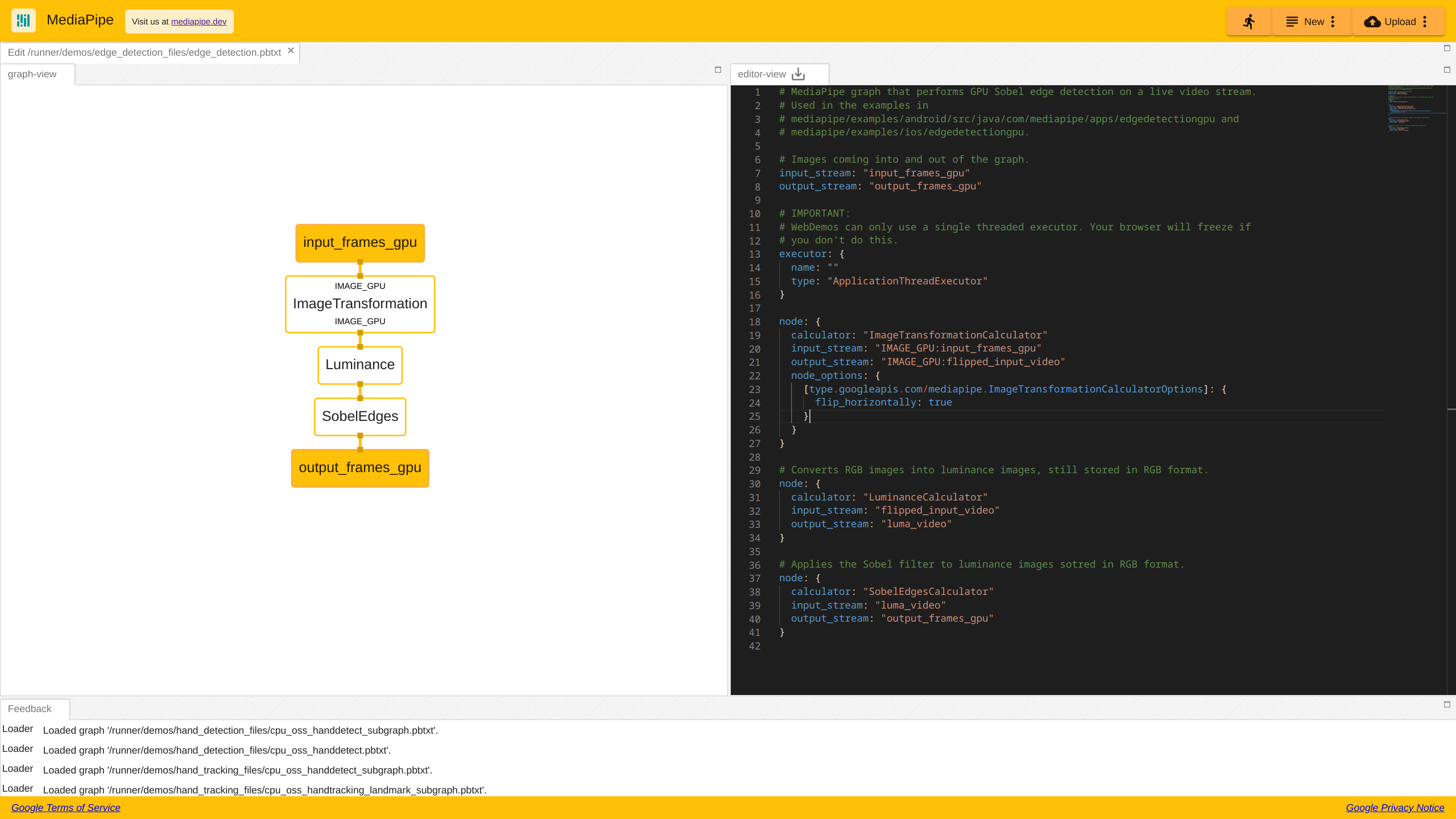
The figure below illustrates a mediapipe graph for performing edge detection on the GPU. Each calculator receives GPU image packets and schedules execution on the available device.
Difference 2: packets and graph scheduling
A packet in Mediapipe is an independent piece of data that travels through the calculator graphs. This enables Mediapipe to schedule running several calculators concurrently, thus potentially increasing performance.
In Lluvia, nodes connected through inputs and outputs do not allocate new memory on each run of the node. Instead, all the memory is allocated at node initialization time, and exposed through the node’s ports. Then, the whole graph is scheduled to run on the GPU device in one go. This reduces the delay in computations as avoids cross-talk between the host CPU and the GPU to synchronize individual node execution.
Lluvia as a mediapipe dependency
Mediapipe, as well as Lluvia, are built using Bazel. As a consequence, the integration of Lluvia can be done by including the project as a Bazel dependency into Mediapipe repository. The current approach to achieve this is through the use of an auxiliary repository, lluvia-mediapipe, that contains the LluviaCalculator node to run GPU compute-pipelines as a Mediapipe calculator. The build instructions are available in the mediapipe integration guide. The process is as follows:
- Clone Mediapipe repository alongside Lluvia.
- Configure Mediapipe’s Bazel workspace to build in your host machine.
- Include Lluvia as a dependency to Mediapipe.
- Clone
lluvia-mediapiperepository inside Mediapipe to enable building its targets. - Run the tests included in the repository to validate the build.
The directory structure of the three projects should look like this:
lluvia                          <-- lluvia repository
mediapipe                       <-- mediapipe repository
├── BUILD.bazel
├── LICENSE
├── ...
├── mediapipe                   <--
│   ├── BUILD
│   ├── calculators
│   ├── examples
│   ├── framework
│   ├── gpu
│   ├── ...
│   ├── lluvia-mediapipe        <-- lluvia-mediapipe repository
├── ...
├── .bazelrc
└── WORKSPACE
Once Mediapipe builds correctly, it is possible to create graphs that include the LluviaCalculator.
The LluviaCalculator
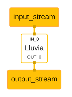
The LluviaCalculator is in charge of initializing Lluvia, binding input and output streams from mediapipe to lluvia ports, and running a given compute pipeline.
The figure below illustrates a basic mediapipe graph utilizing lluvia, while the code below shows the graph description using Protobuffer text syntax:
| |
where:
- The
enable_debugflag tells whether or not the Vulkan debug extensions used by Lluvia should be loaded during session creation. This flag might be set tofalsein production applications to improve runtime performance. - The
library_pathdeclare paths to node libraries (a.zipfile) containing Lluvia nodes (Container and Compute). This attribute can be repeated several times. - The
script_pathis the path to aluascript declaring aContainerNodethat Lluvia will instantiate as the “main” node to run inside the calculator. input_port_binding, maps mediapipe input tags to the mainContainerNodeport. In the example above, mediapipe’s input tagIN_0is mapped to lluvia’sin_imageport.
Examples
lluvia-mediapipe includes two applications, single_image and webcam to run on the host system. The single_image app, as the name suggests, reads the content of a single image and feeds it to a Mediapipe graph.
The command below executes the binary with a graph configured to run the lluvia/color/BGRA2Gray compute node to convert from the BGRA input to gray scale:
| |
where ${HOME}/git is the base folder where Lluvia and Mediapipe are cloned. Change this according to your setup.
A more sophisticated example is running the Horn and Schunck optical flow algorithm inside of Mediapipe. The webcam binary opens the default capture device using OpenCV and transfers the captured frames the compute graph. The graph is a single LluviaCalculator running several nodes:
| |
where --graph_file=${HOME}/git/mediapipe/mediapipe/lluvia-mediapipe/examples/desktop/graphs/HornSchunck/graph.pbtxt is the path to Mediapipe’s graph to be run by the app, and --script_file=${HOME}/git/mediapipe/mediapipe/lluvia-mediapipe/examples/desktop/graphs/HornSchunck/script.lua points to a Lua script defining the Container node to run inside of the LluviaCalculator.
@startuml
skinparam linetype ortho

state LluviaCalculator as "LluviaCalculator" {

    state input_stream as "IN_0:input_stream" <<inputPin>>
    state output_stream as "OUT_0:output_stream" <<outputPin>>

    state ContainerNode as "mediapipe/examples/HornSchunck" {

        state in_image <<inputPin>>

        state BGRA2Gray
        state HS as "HornSchunck"
        state Flow2RGBA
        state RGBA2BGRA

        input_stream -down-> in_image

        in_image -down-> BGRA2Gray
        BGRA2Gray -down-> HS: in_gray
        HS -down-> Flow2RGBA: in_flow
        Flow2RGBA -down-> RGBA2BGRA: in_rgba

        RGBA2BGRA -down-> out_image <<outputPin>>
    }


  out_image -down-> output_stream <<outputPin>>
}

@enduml
First, the input image is transformed from BGRA color space to gray scale. Next, the images are fed to the HornSchunck container node to compute optical flow. The estimated flow is then converted to color using the Flow2RGBA compute node, and finally, the RGBA output is converted to BGRA to proper rendering in the window opened by OpenCV.
Difference 3: calculators as code vs. nodes as data
In Mediapipe, every Calculator must be compiled and integrated into the binary at build time, thus requiring rebuilding every time a new Calculator must be added or modified.
Lluvia describes nodes as a pair of Lua and GLSL (for ComputeNode) files that are compiled and packaged into a node library as a .zip file. Once packaged, the library can be imported on any runtime where Lluvia runs. This eases the developer experience as one can develop nodes in a higher-level environment, using Python in a Jupyter notebook for instance, package the nodes in a node library and then use them in any environment (Mediapipe for instance).
Discussion
This article presented the integration of Lluvia into the Mediapipe project. By added the project into Mediapipe, it is possible to leverage the GPU compute-pipeline capabilities of Lluvia to speed up parts of complex Computer Vision applications.
The integrations between thw two projects is achieved through the LluviaCalculator which runs any arbitrary ContainerNode. This calculator is in early stages of development, and feedback is very welcomed. Some immediate improvements include:
- Support
GPUImageFrameinput and output packets. Currently, the calculator only accepts CPUImageFramepackets, thus introducing some latency while copying data from CPU memory space to the GPU. - Support Mediapipe side packets to send configuration updates to the calculator.
- Include more configuration attributes (e.g. node parameters) in the Protobuffer type.
And finally, testing the integration in other platforms such as Android.
References
Camera undistort
Jupyter notebook:
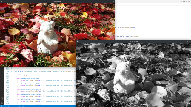
A Jupyter notebook with the code in this article is available in Google Colab. Check it out!Background
Camera undistort is the process by which distortions generated by the optics used in the camera during the capture process are corrected in software. The process requires a mathematical model of the distortion, and a calibration procedure to estimate the parameters of such model given actual images.
An overview of the camera modeling is pressented in the Computer Vision book of Szeliski and the Multiple View Geometry book of Hartley and Zisserman, as well as the articles of Zhang, Wei and Ma.
There are several calibration toolboxes available for estimating the camera model from a series of images:
Any of such frameworks can be used to estimate the camera model parameters. Those parameters are the input to the undistort method presented in this article to rectify raw captured images.
Camera model
The figure below illustrates the camera model.

The 3D point $\mathbf{x} \in \mathbb{R}^3$ is expressed relative to the camera body fixed frame. It projects onto the camera image plane as pixel $\mathbf{p} := (u, v)^\top \in \mathbb{R}^2$ as
$$ \begin{equation} \begin{pmatrix} \mathbf{p} \\ 1 \end{pmatrix} := \begin{pmatrix} u \\ v \\ 1 \end{pmatrix} = \frac{\mathbf{K} \mathbf{x}}{ \left< e_3, \mathbf{x} \right>} \end{equation} $$
where $\mathbf{K} \in \mathbb{R}^{3\times3}$ is the camera intrinsics matrix, $e_3 := (0, 0, 1)^\top$, and $\left< e_3, \mathbf{x} \right>$ is the dot product between the two vectors. The units of $\mathbf{p}$ are actual pixel coordinates in the ranges $u \in [0, W)$ and $v \in [0, H)$, with $W$ and $H$ denoting the image width and height respectively.
Given a pixel point, the corresponding 3D coordinate $\bar{\mathbf{x}}$ in the image plane is defined as:
$$ \begin{equation} \bar{\mathbf{x}} := \begin{pmatrix} \bar{x} \\ \bar{y} \\ \bar{z} \\ \end{pmatrix} = \mathbf{K}^{-1} \begin{pmatrix} \mathbf{p} \\ 1 \end{pmatrix} \end{equation} $$
Standard distortion model
The standard distortion model is formed by two components:
- A radial component parameterized by three coefficients: $k_1$, $k_2$, and $k_3$.
- A tangential component with two parameters: $p_1$ and $p_2$.
The radial distortion component for a given pixel $\mathbf{p}$ is computed as
$$ \begin{equation} \bar{\mathbf{x}}_r := R \begin{pmatrix} \bar{x} \\ \bar{y} \\ 0 \end{pmatrix} \end{equation} $$
where $R \in \mathbb{R}$ is
$$ \begin{equation} R = k_1 r^2 + k_2 r^4 + k_3 r^6 \end{equation} $$
with
$$ \begin{equation} r^2 = \bar{x}^2 + \bar{y}^2 \end{equation} $$
and $\bar{x}, \bar{y}$ are the $x$ and $y$ coordinates of the projection of pixel $\mathbf{p}$ using equation (2).
The tangential distortion is computed as:
$$ \begin{equation} \bar{\mathbf{x}}_p := \begin{pmatrix} 2 p_1 \bar{x}\bar{y} + p_2(r^2 + 2\bar{x}^2) \\ p_1(r^2 + 2 \bar{y}^2) + 2 p_2 \bar{x}\bar{y} \\ 0 \end{pmatrix} \end{equation} $$
Finally, the undistorted image plane coordinates $\bar{\mathbf{x}}_u$ is computed as:
$$ \begin{equation} \bar{\mathbf{x}}_u = \bar{\mathbf{x}} + \bar{\mathbf{x}}_r + \bar{\mathbf{x}}_p \end{equation} $$
Given $\bar{\mathbf{x}}_u$, the corresponding undistorted pixel coordinate is:
$$ \begin{equation} \begin{pmatrix} \mathbf{p}_u \\ 1 \end{pmatrix} := \begin{pmatrix} u_u \\ v_u \\ 1 \end{pmatrix} = \frac{\mathbf{K} \bar{\mathbf{x}}_u}{ \left< e_3, \bar{\mathbf{x}}_u \right>} \end{equation} $$
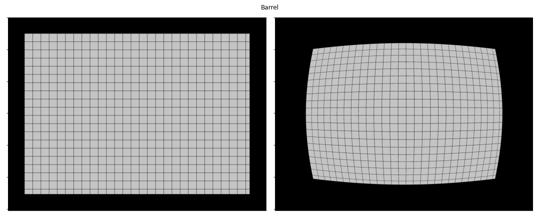
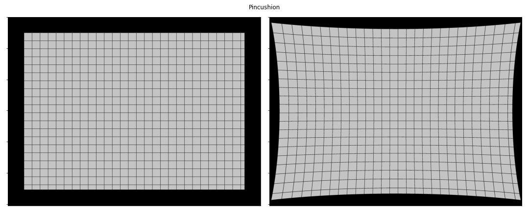
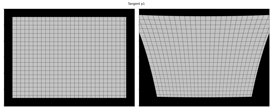
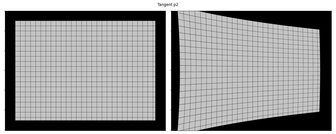
The figures below illustrate the effects of the radial and tangential distortion. A possitive value of $k_1$ creates a barrel effect, while a negative value generates a pincushion effect. For the tangential parameters, $p_1$ models missalignment between the image sensor and the image plane in the $y$ axis, while $p_2$ models such missalignment in the $x$ axis.
Implementation
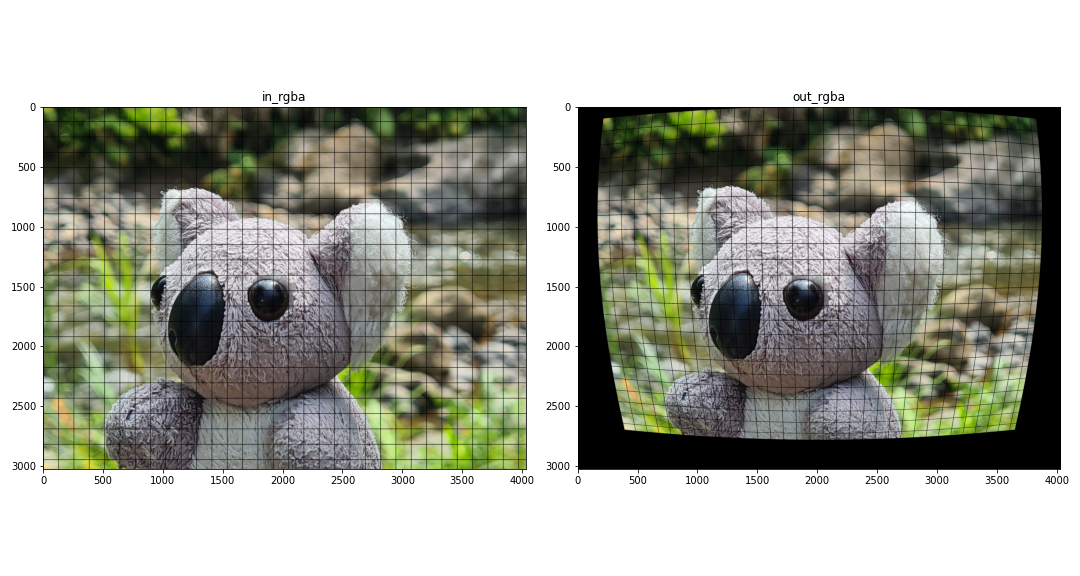
The camera undistort procedure is implemented as a single ComputeNode with the following interface:
@startuml
skinparam linetype ortho

state CameraUndistort as "CameraUndistort_rgba8ui" {

    state in_rgba <<inputPin>>
    state in_camera <<inputPin>>
    state out_rgba <<outputPin>>

}

note top of CameraUndistort
Parameters
----------
camera_model : int. Defaults to 0.
    The camera model used for rectifying the image. Possible values are:

    * 0: standard model
end note

@enduml
The node explicitly requires rgba8ui images to be bound to the node. The output out_rgba is allocated by the node. The in_camera is a UniformBuffer storing the camera model. This model is defined by the ll_camera struct in GLSL as:
| |
Uniform buffers are a special type of buffers used to store small data structures used in graphics and compute pipelines. The Vulkan tutorial on Uniform Buffers is a good read on how they are used in general. Notice that the ll_camera uses GLSL types such as mat3 and vec4. In the host CPU, one must use corresponding types and follow the byte alignmnet rules to make the buffer usable in the GPU. The alignment rules are defined by the STD140 layout rules. For the ll_camera struct, the mat3 attributes must be transferred as a matrix of 4 rows and 3 columns in order to meet the alignment requirements.
Matrix storage in GLSL
In GLSL, matrices are stored in column-major order. For a given matrixM indexed as M[i, j] where i and j are the row and column indexes, respectively, the elements M[i, j] and M[i, j+1] are stored contiguously in memory. This is different, for instance, to numpy’s default ordering as row-major.The code block below shows a complete example on how to run the lluvia/camera/CameraUndistort_rgba8ui node using a dummy camera model with radial and tangential distortion:
| |
Lines 36 to 60 create the uniform buffer containing the camera model. Lines 42 and 45 create the camera intrinsics matrix K and its inverse Kinv. Then, in lines 50-51, those matrices are aligned to meet the std140 requirements; in this case, storing each matrix in a 4x3 matrix in column-major ordering (using order='F' in numpy). Finally, lines 54-55 concatenates all camera parameters to create a single numpy array npBuf which is then used to create the in_camera uniform buffer in lluvia.
Runtime performance
A Razer Blade laptop running Ubuntu 22.04LTS was used for the runtime analysis. The laptop is equipped with an Intel i7-11800H processor, and the following Vulkan devices as reported by the code block below:
| |
- NVIDIA GeForce RTX 3070 Laptop GPU.
- Intel(R) UHD Graphics (TGL GT1).
- llvmpipe (LLVM 13.0.1, 256 bits). This is a CPU implementation of the Vulkan API shipped with the Mesa drivers.
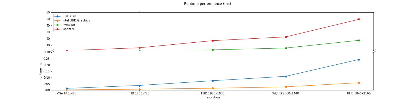
In addition, the cv2.undistort() function from OpenCV is considered for reference. Five resolutions are used in the evaluation: VGA 640x480, HD 1280x720, FHD 1920x1080, WQHD 2560x1440, and UHD 3840x2160. For each resolution, the algorithm is run for 1000 iterations and the median runtime is extracted. The figure and table belows show the runtime for each device and resolution combination.
| Resolution | Device name | Runtime median ms |
|---|---|---|
| VGA 640x480 | Intel UHD Graphics | 0.00235 |
| RTX 3070 | 0.013888 | |
| llvmpipe | 0.604263 | |
| OpenCV | 2.04252 | |
| HD 1280x720 | Intel UHD Graphics | 0.007734 |
| RTX 3070 | 0.03728 | |
| llvmpipe | 1.50221 | |
| OpenCV | 6.38165 | |
| FHD 1920x1080 | Intel UHD Graphics | 0.0151045 |
| RTX 3070 | 0.07456 | |
| llvmpipe | 3.17916 | |
| OpenCV | 17.1453 | |
| WQHD 2560x1440 | Intel UHD Graphics | 0.0262145 |
| RTX 3070 | 0.109344 | |
| llvmpipe | 5.97528 | |
| OpenCV | 22.8469 | |
| UHD 3840x2160 | Intel UHD Graphics | 0.058583 |
| RTX 3070 | 0.242688 | |
| llvmpipe | 17.6178 | |
| OpenCV | 49.477 |
Integrated vs Discrete GPU performance
Notice that the Intel UHD Graphics device reports lower runtime than the discrete Nvidia RTX 3070 GPU. It is not clear why this is the case, as the Nvidia GPU has more compute resources than the Intel integrated graphics.Also, notice how the llvmpipe CPU device is between three to four times faster than the OpenCV function. However, both CPU devices are 2 orders of magnitude slower than the Nvidia and Intel GPU devices.
Discussion
This post showed how to run the camera undistort node in Lluvia. The node takes as input an RGBA image and a camera model stored in a uniform buffer in the GPU, and produces an RGBA output image. The camera model stored in the uniform model must follow the GLSL std140 layout rules. In terms of runtime performance, the GPU implementation is several orders of magnitude faster than the OpenCV default implementation.
Future pieces of work includes:
- Expose the interpolation coordinates for undistorting the images as a new compute node. These coordinates could be cached in order to save computations on every node invocation.
- Clip the undistorted image to a given area according to the camera model. This will be useful to avoid wasted pixels in the output, as shown in the examples.
- Support for more image formats, such as
r8uiand floating point channel types.
References
- OpenCV camera calibration routines.
- Matlab calibration app.
- Vulkan tutorial on Uniform Buffers.
- GLSL STD140 memory layout.
- Mesa llvmpipe.
- Zhang, Z., 2000. A flexible new technique for camera calibration. IEEE Transactions on pattern analysis and machine intelligence, 22(11), pp.1330-1334. Microsoft Technical Report.
- Wei, G.Q. and De Ma, S., 1994. Implicit and explicit camera calibration: Theory and experiments. IEEE Transactions on Pattern Analysis and Machine Intelligence, 16(5), pp.469-480. DOI.
- Szeliski, R., 2010. Computer vision: algorithms and applications. Springer Science & Business Media. Book.
- Hartley, R. and Zisserman, A., 2003. Multiple view geometry in computer vision. Cambridge university press. Book
Implementing the Horn and Schunck optical flow algorithm
Jupyter notebook:
A Jupyter notebook with the code in this article is available in Google Colab. Check it out!Background
The Horn and Schunck variational method for computing optical flow is one of the seminal works in the field. It introduces the idea of using a global smoothness constrain on the estimated optical flow. This constrain helps the numerical solution to find a good flow estimate even in image regions with poor texture.
Let $\mathbf{E}(x, y, t)$ be the image brightness at point $(x, y)$ and time $t$. Considering the constant brightness assumption, where the change in brightness is zero, that is,
$$ \frac{d \mathbf{E}}{d t} = 0 $$
Taking the partial derivatives over $(x, y, t)$, one has:
$$ \frac{\partial \mathbf{E}}{\partial x} \frac{\partial x}{\partial t} + \frac{\partial \mathbf{E}}{\partial y} \frac{\partial y}{\partial t} + \frac{\partial \mathbf{E}}{\partial t} = 0 $$
For convenience, let:
$$ \begin{align*} \mathbf{E}_x &= \frac{\partial \mathbf{E}}{\partial x} \\ \mathbf{E}_y &= \frac{\partial \mathbf{E}}{\partial y} \\ \mathbf{E}_t &= \frac{\partial \mathbf{E}}{\partial t} \end{align*} $$
be the image gradient in the $x$ and $y$ directions, and the partial derivative in time, respectively, and
$$ \begin{align} u &= \frac{\partial x}{\partial t} \\ v &= \frac{\partial y}{\partial t} \end{align} $$
be the $x$ and $y$ components of the optical flow, respectively. The constant brightness equation is then
$$ \mathbf{E}_x u + \mathbf{E}_y v + \mathbf{E}_t = 0 $$
which is the basis for the differential methods for computing optical flow (e.g. Lukas-Kanade).
Minimization
Differential methods for estimating optical flow try to minimize the cost function
$$ \epsilon_b = \mathbf{E}_x u + \mathbf{E}_y v + \mathbf{E}_t $$
that is, to try to find values $(u, v)$ of the optical flow such that the constant brightness constrain is maintained. Notice that there is a single cost funcion and two unknowns $(u, v)$. To solve this, the Horn and Schunck algorithm adds a smoothness constrain based on the average value of the flow in a neighborhood, as
$$ \epsilon_c^2 = (\bar{u} - u )^2 + (\bar{v} - v)^2 $$
Combining both cost functions, one has
$$ \epsilon^2 = \alpha^2 \epsilon_b^2 + \epsilon_c^2 $$
From these equations, a numerical solution is derived. The reader is encouraged to go to the paper for more details. The iterative solution for $(u, v)$ is
$$ \begin{align*} u^{n+1} &= \bar{u}^n - \mathbf{E}_x \frac{\mathbf{E}_x \bar{u}^n + \mathbf{E}_y \bar{v}^n + \mathbf{E}_t}{\alpha^2 + \mathbf{E}_x^2 + \mathbf{E}_y^2} \\ v^{n+1} &= \bar{v}^n - \mathbf{E}_y \frac{\mathbf{E}_x \bar{u}^n + \mathbf{E}_y \bar{v}^n + \mathbf{E}_t}{\alpha^2 + \mathbf{E}_x^2 + \mathbf{E}_y^2} \end{align*} $$
where $(u^{n+1}, v^{n+1})$ is the estimated optical flow at iteration $n + 1$, using the estimated flow at previous iterations and image parameters computed from an image pair.
Implementation
The figure below illustrates the pipeline implementing the algorithm:
@startuml
skinparam linetype ortho

state HS as "HornSchunck" {

  state in_gray <<inputPin>>

  state ImageProcessor
  state ImageNormalize_uint_C1

  state NI_1 as "NumericIteration 1"
  state NI_2 as "NumericIteration 2"
  state NI_3 as "NumericIteration 3"
  state NI_N as "NumericIteration N"

  in_gray -down-> ImageProcessor
  in_gray -down-> ImageNormalize_uint_C1


  ImageNormalize_uint_C1 -down-> ImageProcessor: in_gray_old

  ImageProcessor -down-> NI_1: in_image_params
  ImageProcessor -down-> NI_2
  ImageProcessor -down-> NI_3
  ImageProcessor -down-> NI_N: in_image_params

  NI_1 -> NI_2
  NI_2 -> NI_3
  NI_3 -> NI_N: ...
  NI_N -> NI_1: in_flow, used for next image iteration

  NI_N -down-> out_flow <<outputPin>>
  ImageNormalize_uint_C1 -down> out_gray <<outputPin>>
}

note top of HS
Parameters
----------
alpha : float. Defaults to 0.05.
    Regularization gain.

iterations : int. Defaults to 1.
    Number of iterations run to compute the optical flow.

float_precision : int. Defaults to ll.FloatPrecision.FP32.
    Floating point precision used accross the algorithm. The outputs out_gray
    and out_flow will be of this floating point precision.
end note
@enduml
The HornSchunck is a ContainerNode that instantiates several ComputeNode implementing the algorithm. In particular, the ImageProcessor node computes image parameters from the pair of images in_gray and in_gray_old. Those parameters are transfered to the instances of NumericIteration through in_image_params, organized as follows:
in_image_params.x: X component of the image gradientin_image_params.y: Y component of the image gradientin_image_params.z: temporal derivative betweenin_grayandin_gray_old.in_image_params.w: gain for this pixel computed from image gradient andalphaparameter.
This packaging of the image parameters is convenient as all values are packed together in a singe RGBA pixel. The floating point precision of this, and the estimated optical flow is controlled by the float_precision parameter.
The NumericIteration node takes the image parameters and a prior estimation of the optical flow, in_flow, and computes the next iteration of the flow field. The algorithm requires several iterations for the estimated flow to be of acceptable quality. In the figure above, the last iteration is denoted as NumericIteration_N and it feeds its output back as input to the first one, as well as the output of the HornSchunck node. The number of iterations is controlled by the iterations parameter.
The code block below shows how to run a simple pipeline:
@startuml
skinparam linetype ortho

state RGBA2Gray
state HS as "HornSchunck"
state Flow2RGBA

RGBA2Gray -down-> HS: in_gray
HS -down-> Flow2RGBA: in_flow
@enduml
where RGBA2Gray converts an input RGBA image to gray scale, HornSchunck computes the optical flow, and Flow2RGBA converts the optical flow to color representation.
| |
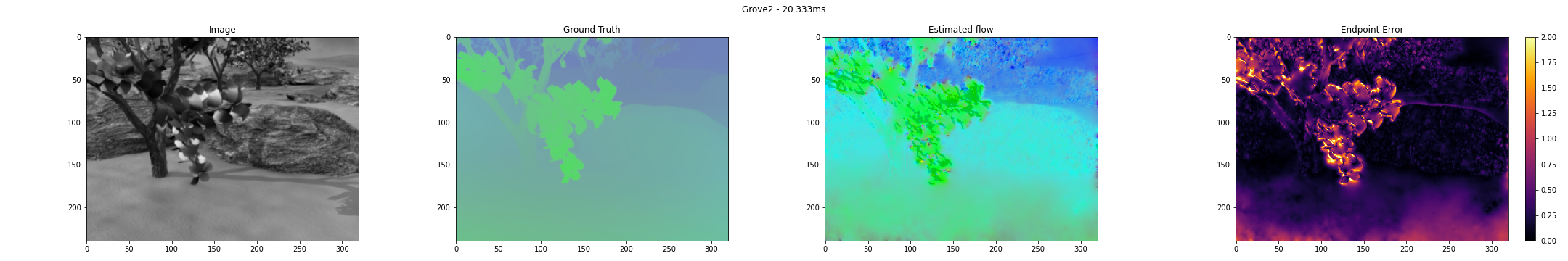
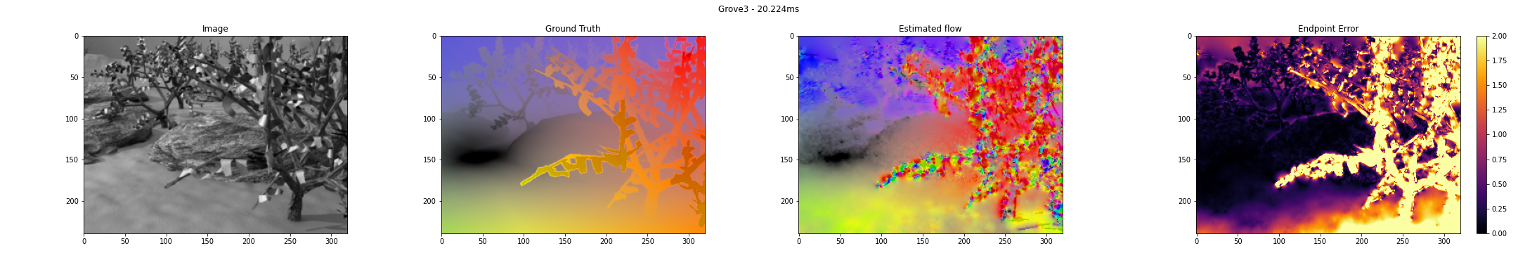
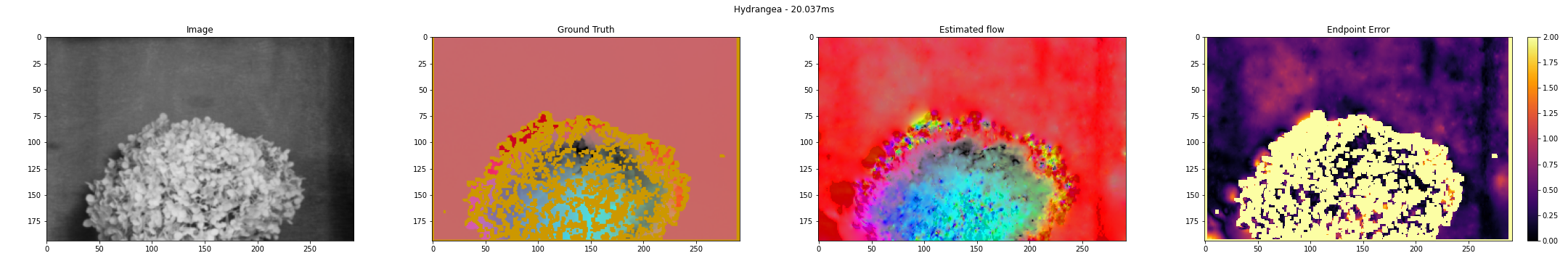
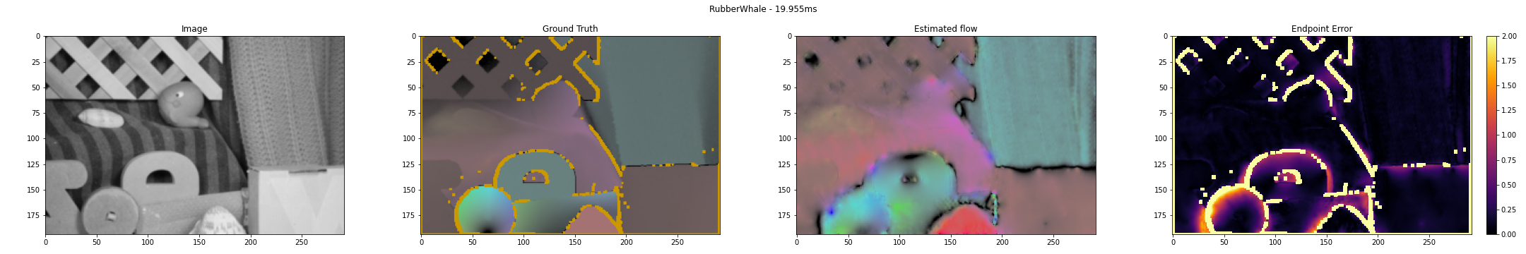
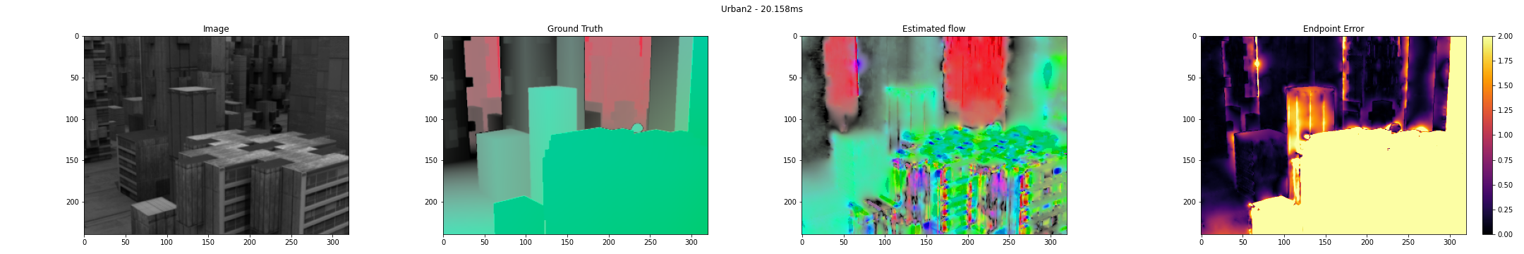
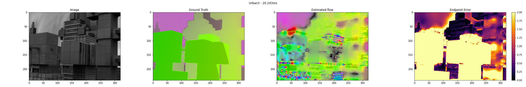
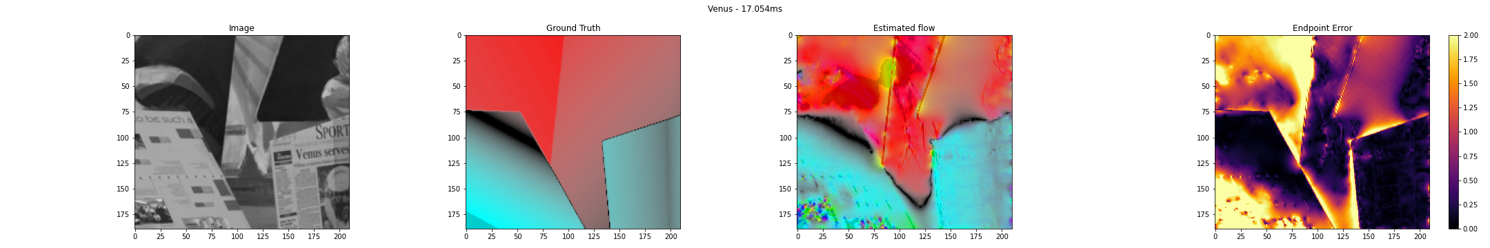
Evaluation on the Middlebury dataset
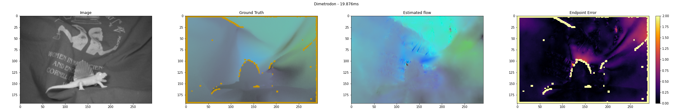
The Middlebury optical flow dataset from Baker et. al. provides several real-life and synthetic image sequences with ground truth optical flow. The figures below shows the estimated optical flow for the test sequences whose ground truth is available.
The Horn ans Schunck algorithm is not well suited for large pixel displacements. Considering this, the input images are scaled to half before entering the compute pipeline. The ground truth flow is scaled accordingly in order to be compared with the estimated flow. The Endpoint Error measures the different in magnitude between the ground truth and the estimation, it is computed as:
$$ EE = \sqrt{(u - u_\text{gt})^2 + (v - v_\text{gt})^2} $$
The algorithm is configured as follows:
alpha: 15.0/255iterations: 2000float_precision: FP32
In general, the estimated optical flow yields acceptable results in image regions with small displacements (e.g. Dimetrodon, Grove2, Hydrangea, and RubberWhale). In image regions with large displacements, the method is not able to compute a good results, as can be visualized in the Urban2 and Urban3 sequences.
The results reported in this post were run on a Razer Blade 2021 Laptop equipped with an Nvidia RTX 3070 GPU. The runtime is reported in the title of each figure, and is in the order of 20 milliseconds for most of the image sequences. Section runtime performance evaluates the performance of the algorithm on different devices, resolutions, and floating point precisions.
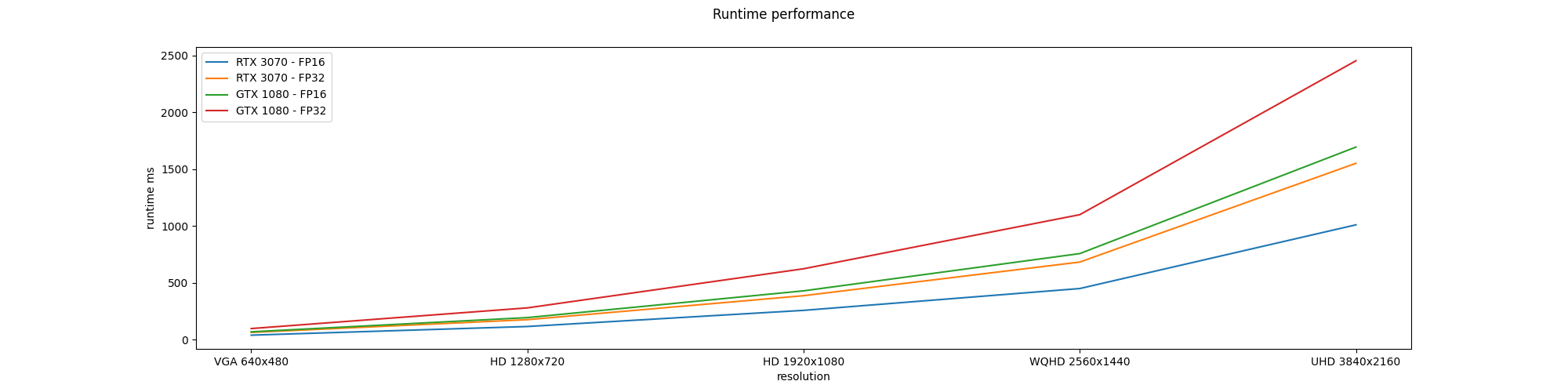
Runtime performance
For the runtime analysis of the algorithm, two GPU devices were used:
- A Nvidia GTX 1080 Desktop GPU.
- A Nvidia RTX 3070 Laptop GPU running on a Razer Blade 2021.
The Horn and Schunck pipeline is configured using the same number of iterations used for the Middlebury evalatuon, that is, iterations = 2000. The pipeline is configured for 5 different image resolutions (VGA 640x480, HD 1280x720, HD 1920x1080, WQHD 2560x1440, UHD 3840x2160). For each resolution, the pipeline is run both using FP16 and FP32 floating point precision. The table and figure below show the runtime performance for each configuration.
| Resolution | Float precision | Device | Runtime median (ms) |
|---|---|---|---|
| VGA 640x480 | FP16 | GTX 1080 | 68.8196 |
| RTX 3070 | 39.4354 | ||
| FP32 | GTX 1080 | 97.5005 | |
| RTX 3070 | 63.6458 | ||
| HD 1280x720 | FP16 | GTX 1080 | 193.977 |
| RTX 3070 | 115.626 | ||
| FP32 | GTX 1080 | 279.538 | |
| RTX 3070 | 175.635 | ||
| HD 1920x1080 | FP16 | GTX 1080 | 429.256 |
| RTX 3070 | 257.624 | ||
| FP32 | GTX 1080 | 623.555 | |
| RTX 3070 | 386.718 | ||
| WQHD 2560x1440 | FP16 | GTX 1080 | 757.101 |
| RTX 3070 | 449.536 | ||
| FP32 | GTX 1080 | 1099.35 | |
| RTX 3070 | 682.558 | ||
| UHD 3840x2160 | FP16 | GTX 1080 | 1694.16 |
| RTX 3070 | 1010.16 | ||
| FP32 | GTX 1080 | 2453.45 | |
| RTX 3070 | 1551.34 |
It is not surprising that the RTX 3070 GPU is faster than the GTX 1080, as the former is of a newer generation than the latter.
Discussion
This post presented a GPU implementation of the Horn and Schunck optical flow algorithm. Evaluation in the Middlebury test sequences show the validity of the implementation. A runtime performance analysis was conducted on two GPUs using several image resolutions and floatin point precisions.
Future work includes:
- Implementing a pyramidal scheme, for instance that of Llopis et. al., to improve the accuracy of the algorithm in presence of large displacements.
- Use the smoothness constrain and numerical scheme in the FlowFilter algorithm to improve the accuracy.
References
- Horn, Berthold KP, and Brian G. Schunck. “Determining optical flow.” Artificial intelligence 17.1-3 (1981): 185-203. Google Scholar.
- Baker, S., Scharstein, D., Lewis, J.P., Roth, S., Black, M.J. and Szeliski, R., 2011. A database and evaluation methodology for optical flow. International journal of computer vision, 92(1), pp.1-31. Google Scholar.
- Meinhardt-Llopis, E. and Sánchez, J., 2013. Horn-schunck optical flow with a multi-scale strategy. Image Processing on line. Google Scholar
- Adarve, Juan David, and Robert Mahony. “A filter formulation for computing real time optical flow.” IEEE Robotics and Automation Letters 1.2 (2016): 1192-1199. Google Scholar
Working with floating point precision
Jupyter notebook:
A Jupyter notebook with the code in this article is available in Google Colab. Check it out!GPU devices support several floating point number precisions, where precision refers to the number of bits used for representing a given number. Typical representations are:
FP16: or half precision. Numbers are represented in 16 bits.FP32: or single precision. It uses 32 bits for representing a number.FP64: or doble precision. 64 bits are used for represeting a number.
FP64 is used when numerical precision is required, while FP16 is suitable for fast, less exact calculations, and FP32 sits in the middle. The IEEE 754 standard defines the specification of floating point numbers used in modern computers. It defines the rules for interpreting the bit fields that form a number, as well as the arithmetic rules to process them.
The Vulkan API offers support for the three floating point precisions. However, not all GPUs support every format. The Vulkan GPU Info page is great tool to check support for a given feature.
Improvements in runtime performance
Smaller bit representation of floating point numbers have an advantage in terms of runtime performance. Consider the case of a RGBA image. If the image channel type is ll.ChannelType.Float16, the four pixel values will fit in 8 bytes, compared to the 16 bytes needed if ll.ChannelType.Float32 was used. This reduction in memory footprint increases the pixel transfer rate from memory to the compute device.
To illustrate this, let’s consider the optical flow filter node. The code below configures the flowfilter algorithm both with ll.FloatPrecision.FP16 and ll.FloatPrecision.FP32, it runs each node for N = 10000 iterations and collects its runtime using the duration probe.
| |
Here, the ll.FloatPrecision.FP16, ll.FloatPrecision.FP32 are new enum values for representing 16-bit and 32-bit floating point precision, respectively. The line flowFilter.setParameter('float_precision', ll.Parameter(precision.value)) configures the node with the given precision. Internally, the float_precision is used to instantiate any floating point image with the requested precision.
Note:
By convention, any node that allows selecting floating point precision will define thefloat_precision parameter and will expect one of the ll.FloatPrecision enum values.The figure below shows the collected runtime for both floating point precisions. The median runtime for FP16 is 0.501ms, while for FP32 is 0.770ms. That is, the FP16 algorithm improves the runtime by 35% compared to FP32.
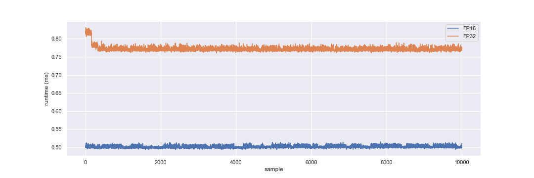
Optical flow filter runtime using FP16 and FP32 floating point precision. Results collected on a Nvidia GTX-1080 (driver 460.91.03) running Ubuntu 20.04.
Modifications to GLSL shader code
In terms of GLSL shader code, there are no changes to support FP16 or FP32 images. However, it is important to understand the underlying functioning. For instance, consider the GLSL implementation of the RGBA2HSVA compute node. Notice that the out_hsva port is bound to the shader as a rgba32f image:
| |
Images compatible with the rgba32f image format can be bound as output. The shader image load store extension defines the compatibility rules to be able to bind images to shaders. For this case in particular, it is possible to bind either a rgba16f or rgba32f images to the output. The shader will execute all arithmetic operations using 32-bit floating point precision. When storing an image texel using imageStore(out_hsva, coords, HSVA), the shader will reinterpret the vec4 HSVA either as a 16 or 32-bit floating vector, according to the image bound to out_hsva.
In terms of Lua code to build the node, these are the considerations to support different precisions:
- Define the
float_precisionparameter with default value toll.FloatPrecision.FP32. - Allocate the node objects according to the selected precision.
In the code below, line local outImageChannelType = ll.floatPrecisionToImageChannelType(float_precision) transforms the recevied ll.FloatPrecision value to the corresponding ll.ChannelType. Then, out_hsva is created and bound to the node.
| |
Discussion
There are several floating point precisions available to use in compute shaders: FP16, FP132, and FP64, are the ones more commonly available in commodity GPU hardware. The ability to control the underlying floating point precision used in compute pipelines can improve runtime performance, as the transfer rate of data from and to memory can increase. The choice of a given precision must be made carefully, as it might affect the accuracy of the algorithm.